
Geometric Dimensioning and Tolerancing (GD&T) is a vital language in the realm of engineering and manufacturing, serving as a set of symbols and principles that convey precise specifications for the design and production of mechanical components. GD&T plays a crucial role in enhancing communication between designers, engineers, and manufacturers, ensuring that everyone involved in the process interprets design intent accurately. Understanding the Basics of GD&T At its core, GD&T is a symbolic language that allows designers to communicate geometric characteristics and tolerances more precisely than traditional methods. Unlike traditional dimensioning, which primarily focuses on size, GD&T incorporates symbols and annotations to convey information about form, orientation, location, and runout. The fundamental elements of GD&T include: Symbols: GD&T uses a set of symbols to represent various geometric characteristics and tolerances. Common symbols include position, concentricity, perpendicularity, and parallelism. Datums: Datums are reference points or planes that serve as the basis for measurements and tolerances. They establish the coordinate system for the part. Feature Control Frames: These frames encapsulate the GD&T symbols and provide a compact way to communicate the desired tolerances and geometric characteristics for a specific feature. Importance of GD&T in Engineering Drawings GD&T is essential for several reasons: Precision and Clarity: GD&T provides a clear and precise way to communicate design requirements. This minimizes ambiguity and reduces the likelihood of misinterpretation. Uniformity: Standardizing on GD&T promotes consistency across design and manufacturing processes, ensuring that everyone in the supply chain understands and adheres to the specified tolerances. Cost Reduction: By accurately defining tolerances, GD&T helps optimize manufacturing processes, reducing the likelihood of defects and rework. This, in turn, lowers production costs. Global Compatibility: GD&T is an internationally recognized standard, making it easier for companies to collaborate on a global scale. Engineers and manufacturers worldwide can understand and implement GD&T specifications. Getting Started with GD&T For beginners, delving into GD&T can be a bit overwhelming. However, a solid foundation begins with understanding the basic symbols and concepts. Here are a few key points to kickstart your GD&T journey: Learn the Symbols: Familiarize yourself with symbols such as position, concentricity, perpendicularity, and parallelism. Each symbol conveys specific information about the geometric characteristics of a feature. Understand Datums: Grasp the concept of datums and their role in establishing a reference coordinate system. Datums are crucial for interpreting the tolerances specified in a drawing. Explore Feature Control Frames: Practice reading and creating feature control frames. These frames encapsulate the GD&T symbols, making it easier to convey design requirements for individual features. Take Advantage of Resources: Numerous resources, including textbooks, online courses, and software tutorials, are available to help you learn GD&T. Leverage these tools to enhance your understanding and practical application of GD&T principles. In conclusion, GD&T is a powerful tool that elevates the precision and clarity of engineering drawings. Embracing GD&T principles not only enhances communication but also contributes to cost-effective and efficient manufacturing processes. As you embark on your GD&T journey, remember that practice and continuous learning are key to mastering this language of precision in engineering.
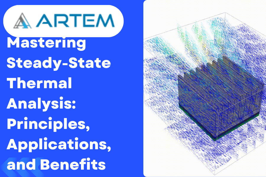
Introduction: In the intricate world of engineering and design, understanding how heat is distributed and managed within structures is paramount. Steady-State Thermal Analysis stands as a powerful tool in this quest, providing engineers with invaluable insights into temperature distributions, heat flow patterns, and the thermal equilibrium of a system. In this blog, we’ll delve into the principles, applications, and benefits of Steady-State Thermal Analysis. 1. Steady State Analysis: In steady-state conditions, temperatures, and heat distributions within a system remain constant over time. This analysis assumes that the system has reached thermal equilibrium, allowing engineers to focus on the long-term behavior of the structure 2. Transient Analysis: In contrast, transient analysis considers changes in temperature over time, exploring how the system responds to dynamic heat inputs or varying thermal conditions. Governing Equations: The fundamental equation governing steady-state thermal analysis is the heat conduction equation: $$\nabla⋅(\nabla)+=0\nabla⋅(k\nabla T)+Q=0$$ Where k is the thermal conductivity, T is the temperature, and Q represents any heat sources or sinks. Conducting Steady-State Thermal Analysis: $$a^2\;+\;b^{2\;}=\;KU$$ Boundary Conditions: Setting appropriate boundary conditions is crucial. Engineers define temperatures, heat fluxes, or convective heat transfer coefficients at different surfaces to simulate real-world scenarios. Material Properties: Accurate representation of material properties, especially thermal conductivity, is essential. Different materials conduct heat at varying rates, impacting how heat is transferred within the structure. Mesh Generation: Discretizing the structure into smaller elements through mesh generation is a key step. A finer mesh allows for a more accurate representation of temperature variations. Solver Selection: Solvers, often finite element analysis (FEA) tools, are employed to solve the complex mathematical equations governing heat transfer. These tools provide temperature distributions and heat fluxes within the structure. Applications of Steady-State Thermal Analysis: 1. Electronics Cooling: Ensuring electronic components operate within temperature limits is critical. Steady-state thermal analysis helps optimize heat sink designs and cooling strategies. 2. Building Thermal Performance: Evaluating how heat is transferred through building materials aids in designing energy-efficient structures. This analysis is crucial for assessing insulation requirements and HVAC system sizing. 3. Automotive Engineering: In the automotive industry, steady-state thermal analysis is employed to prevent overheating of components, optimize radiator designs, and enhance overall vehicle thermal performance. 4. Industrial Equipment: Efficient operation of industrial machinery often relies on steady-state thermal analysis to prevent overheating and optimize heat dissipation mechanisms. Benefits of Steady-State Thermal Analysis: 1. Optimization of Designs: Engineers can fine-tune designs to ensure that components operate within temperature limits, maximizing efficiency and longevity. 2. Cost Savings: By identifying potential overheating issues early in the design process, unnecessary costs associated with redesign and system failures can be avoided. 3. Energy Efficiency: Steady-state thermal analysis contributes to the development of energy-efficient systems by optimizing insulation, cooling, and heating strategies. Conclusion: Steady-state thermal analysis is an indispensable tool for engineers navigating the complex world of heat transfer. From electronics to buildings and industrial machinery, the insights gained from this analysis play a pivotal role in optimizing designs, ensuring reliability, and fostering innovation in diverse engineering domains. As technology advances, the application of steady-state thermal analysis continues to shape the way we harness and manage heat in the pursuit of safer, more efficient, and resilient systems.

Welcome, aspiring engineers and graduate students! As you delve into the intricate world of Computer-Aided Design (CAD), mastering tools like Siemens NX can be a game-changer. Today, let’s unravel the secrets of NX CAD workflow optimization, a journey that promises not just efficiency but a heightened level of productivity in your design endeavors. Understanding the NX CAD Ecosystem Before we dive into optimization strategies, let’s briefly explore what makes Siemens NX a powerhouse in the CAD realm. NX offers a comprehensive suite of tools for 3D modeling, simulation, and manufacturing. It’s renowned for its parametric design capabilities, advanced simulation tools, and seamless integration across various stages of the product development lifecycle. The Quest for Optimization 1. Mastering Parametric Design: Siemens NX thrives on parametric modeling, where relationships between elements are defined. Embrace the power of design intent by leveraging parameters, constraints, and equations. Establishing a robust parametric foundation not only ensures design flexibility but also expedites modifications when your project evolves. 2. Harnessing Synchronous Technology: NX’s Synchronous Technology is a game-changer. This feature allows for direct editing of 3D models without the need for a history tree. Learn to leverage this tool for quick design changes, reducing the need to backtrack through a sequence of operations. It’s the key to nimble and adaptive design practices. 3. Effective Use of Assemblies: As your projects grow in complexity, mastering assembly design becomes paramount. NX excels in this arena. Learn to use intelligent components, constraints, and motion simulation to optimize your assembly workflow. This ensures efficient collaboration and streamlines the integration of various components into a cohesive product. 4. Utilizing Design Features and Templates: Design features and templates in NX are your productivity allies. Create reusable templates for standard components or assemblies, saving time on repetitive tasks. Understand how to use design features to encapsulate design intent and simplify the creation of complex geometries. 5. Simulation-Driven Design: Siemens NX offers robust simulation tools. Integrate simulation early in your design process to identify potential issues and iterate swiftly. By adopting a simulation-driven design approach, you not only optimize your workflow but also enhance the overall quality of your designs. 6. The Path to Peak Productivity Optimizing your NX CAD workflow is not just about mastering tools; it’s a mindset. As a graduate student, the skills you cultivate now will shape your future endeavors. Embrace continuous learning, explore advanced features, and connect with the vibrant community of NX users. Remember, the key to productivity lies in efficiency, adaptability, and a willingness to explore the vast capabilities of Siemens NX. So, go ahead, unleash your creativity, and let Siemens NX be the canvas for your engineering masterpieces. The world of optimized CAD workflows awaits your innovative touch!
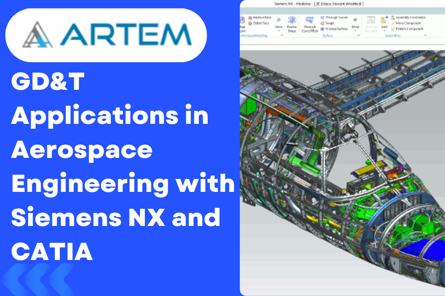
Aerospace engineering stands as a testament to human innovation, pushing the boundaries of what’s possible. At the heart of this cutting-edge industry lies Geometric Dimensioning and Tolerancing (GD&T), a language of precision that ensures every component, no matter how intricate, aligns seamlessly. In this exploration, we’ll delve into real-world case studies, demonstrating how GD&T is intricately woven into aerospace design using CAD tools like Siemens NX and Dassault Systèm CATIA. Case Study 1: Fuselage Alignment in Siemens NX In the design of an aircraft fuselage using Siemens NX, precise alignment is critical for aerodynamics and structural integrity. GD&T plays a pivotal role in ensuring that the various components come together seamlessly. The position control feature in GD&T is employed to define the exact location of critical points on the fuselage concerning a datum reference frame. Example: The GD&T callouts on the blueprint define the position of crucial points, such as mounting brackets and access panels, relative to a specific datum. This precision is vital to maintain the aerodynamic profile and structural stability of the aircraft. Case Study 2: CATIA’s Role in Wing Manufacturing Dassault Systèm CATIA takes center stage in the manufacturing of aircraft wings, where tolerances are incredibly tight. In this scenario, GD&T is used to define not only the dimensions but also the permissible variations in shape, ensuring the wings meet strict performance criteria. Example: The profile of the wing’s airfoil is defined using GD&T in CATIA, ensuring that the curvature and cross-sectional shape conform to the design intent. This meticulous control over the form guarantees optimal lift and drag characteristics during flight. Case Study 3: Aerospace propulsion systems demand unparalleled precision. In the design of engine mounts using Siemens NX, GD&T is employed to guarantee the accurate positioning and alignment of the engine components. Example: GD&T controls are utilized to specify the tolerances for the location of engine mounting points, ensuring that the powerplant aligns precisely with the aircraft’s center of gravity. This level of precision is essential for balanced flight and optimal fuel efficiency. Lessons Learned: The Power of GD&T in Aerospace Design 1. Enhanced Communication: GD&T serves as a universal language, facilitating clear communication between design engineers, manufacturers, and quality control teams. In the aerospace industry, where collaboration is key, this is paramount. 2. Optimized Manufacturing Processes: By defining tolerances and geometric characteristics precisely, GD&T allows for efficient and cost-effective manufacturing processes. This is particularly crucial in aerospace, where components need to meet stringent standards while maintaining a balance between performance and weight. 3. Improved Product Quality: The application of GD&T in aerospace design ensures that every component aligns with design intent, leading to enhanced product quality, increased safety margins, and improved overall performance. In conclusion, GD&T isn’t just a set of symbols on blueprints; it’s the silent force guiding the precision in aerospace engineering. Whether it’s the alignment of fuselage components, the shape of wing profiles, or the positioning of engine mounts, GD&T in conjunction with CAD tools like NX and CATIA is the unsung hero of aerospace design, propelling us to new heights of innovation and reliability.
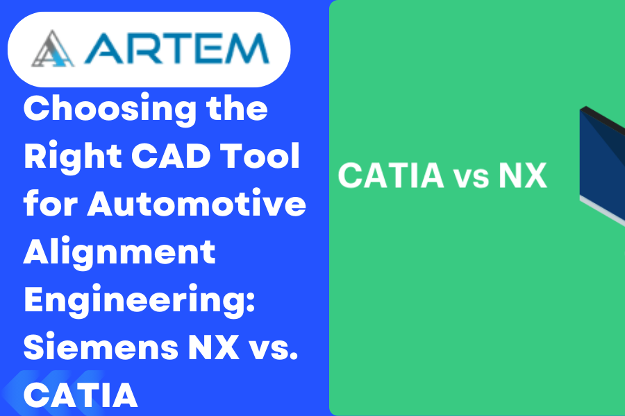
If you’re aspiring to carve your niche in the dynamic world of automotive alignment engineering, mastering Computer-Aided Design (CAD) is a crucial pit stop on your career journey. The question then arises: which CAD software is the best companion for engineers in this field? Buckle up as we navigate through the options and unveil the ideal CAD destination for your automotive alignment career. The CAD Landscape: Navigating the Options The realm of CAD is vast, with various tools catering to different industries and design needs. When it comes to automotive alignment, two major players stand out: Siemens NX and CATIA 1. Siemens NX: Driving Precision and Integration Why Siemens NX? Parametric Modeling Skill: Siemens NX is renowned for its robust parametric modeling capabilities. For automotive alignment engineers, this means the ability to create and modify 3D models with ease, ensuring precise alignment specifications are met. Integrated Simulation: In the automotive world, simulation is key. Siemens NX offers comprehensive simulation tools, allowing engineers to predict and optimize the performance of alignment systems before they hit the road. Collaboration and Integration: Siemens NX seamlessly integrates with other Siemens solutions, providing a unified platform for design, simulation, and manufacturing. This integration ensures a smooth workflow, vital for automotive alignment projects with multidisciplinary requirements. 2. CATIA: Streamlining Complex Designs Why CATIA? Surface Modeling Excellence: CATIA is renowned for its advanced surface modeling capabilities. This is a game-changer for automotive alignment engineers dealing with the sleek and aerodynamic designs of modern vehicles. Collaborative Design: CATIA fosters collaboration, allowing engineers to work concurrently on different aspects of a design. In the context of automotive alignment, where various components must work in harmony, this collaborative feature is invaluable. Industry Dominance: CATIA has a strong presence in the automotive industry, making it a preferred choice for many automotive manufacturers. Learning CATIA can open doors to opportunities in major automotive companies. Choosing Your CAD Vehicle: A Personal Journey The choice between Siemens NX and CATIA ultimately depends on your specific career goals, the industry landscape in your region, and your personal preferences. Here are a few factors to consider: Industry Demand: Research the companies in your region or the ones you aspire to work for. Some may have a preference for Siemens NX, while others might lean towards CATIA. Learning Curve: Both Siemens NX and CATIA have learning curves, but your personal learning style might align better with one over the other. Consider exploring trial versions or introductory courses to get a feel for each. Future Growth: Look into the future development plans of each CAD software. Consider which one aligns with the evolving trends and technologies in the automotive alignment field. Aspect Siemens NX CATIA Industry Adoption Widely used in automotive and aerospace industries. Prevalent in automotive, aerospace, and industrial design. Parametric Modeling Strong parametric modeling capabilities. Robust parametric modeling with advanced features. Surface Modeling Excellent surface modeling for complex designs. Known for advanced and precise surface modeling. Assembly Design Efficient assembly design tools with intelligent components. Powerful assembly design capabilities with collaboration features. Simulation and Analysis Integrated simulation tools for structural, thermal, and fluid analysis. Comprehensive simulation and analysis capabilities. Collaboration Capabilities Seamless integration with Teamcenter for PLM and collaborative design. Collaboration tools facilitate concurrent design among team members. Electrical Systems Design Provides capabilities for electrical systems design. Strong support for electrical systems design and integration. CAM (Computer-Aided Manufacturing) Integrated CAM solutions for manufacturing processes. Extensive CAM tools for a range of manufacturing applications. Industry Standards Compliance Compliant with industry standards like ISO 16792 (STEP AP242). Known for compliance with various industry standards. User Interface User-friendly interface, easier for beginners. Interface design may have a steeper learning curve. Customization and Extensions Extensive customization options and a wide range of extensions. Offers customization options but may have fewer extensions. Cost Consideration Licensing and maintenance costs can be relatively high. Cost structure may vary, and licensing costs can be significant. Conclusion: Steering Toward Success As you rev up your career in automotive alignment engineering, remember that both Siemens NX and CATIA are powerful tools with unique strengths. The best CAD for you is the one that aligns with your career goals, the industry landscape, and your personal preferences. So, buckle up, choose your CAD vehicle wisely, and enjoy the ride toward a successful and fulfilling career in automotive alignment engineering.

Congratulations, graduate! You’re on the tip of diving into the exciting world of Computer-Aided Design (CAD). As you embark on this journey, a critical decision awaits: which CAD tool should you learn to kickstart your career? In this blog, we’ll navigate through the industry landscapes of three prominent CAD tools — SolidWorks, Siemens NX, and CATIA — to help you make an informed choice tailored to your career aspirations. 1. SolidWorks: Bridging Simplicity and Power Industry Recognition: SolidWorks has carved a niche for itself in industries ranging from product design to consumer goods. Its user-friendly interface and ease of learning make it a popular choice, especially for small to mid-sized enterprises. Strengths for Graduates: User-Friendly: SolidWorks is known for its intuitive interface, making it an excellent starting point for beginners. Broad Applicability: Widely used in industries like consumer electronics, medical devices, and general manufacturing, SolidWorks provides versatility. Consider SolidWorks if: You’re looking for an easy entry point into CAD. Your career trajectory is aligned with industries where SolidWorks is extensively used. 2. Siemens NX: Engineering Precision in Motion Industry Recognition: Siemens NX dominates industries with high precision requirements, such as aerospace, automotive, and machinery. It’s the go-to choice for large enterprises and those pushing the boundaries of innovation. Strengths for Graduates: Parametric Design Power: Siemens NX excels in parametric modeling, allowing for complex and precise designs. Comprehensive Simulation: Ideal for graduates interested in simulation-driven design processes. Consider Siemens NX if: You’re aiming for a career in industries demanding high precision, like aerospace or automotive. Your interest lies in comprehensive simulation and engineering analysis. 3. CATIA: For the Architects of Complexity Industry Recognition: CATIA is an industry leader, particularly in aerospace, automotive, and industrial design. It’s a robust choice for handling complex, surface-intensive designs. Strengths for Graduates: Advanced Surface Modeling: CATIA’s surface modeling capabilities are unparalleled, making it a favorite for intricate designs. Collaborative Design: Ideal for graduates aspiring to work on projects with multiple collaborators. Consider CATIA if: You’re fascinated by complex and aesthetically demanding designs. Your career goals align with industries prioritizing collaborative design environments. Making Your Decision: Tailoring CAD to Your Career Path Evaluate Industry Demand: Research the industries prevalent in your region or those you aspire to work in. Identify which CAD tool is in high demand among potential employers. Consider Your Learning Style: Each CAD tool has its learning curve. Consider your learning preferences and explore introductory courses or trial versions to find a tool that aligns with your style. Long-Term Goals: Think about your long-term career goals. If precision engineering and simulation are your interests, Siemens NX might be a good fit. For versatile applications, SolidWorks could be ideal, while CATIA excels in intricate and collaborative design scenarios. Conclusion: Your CAD Journey Begins As you embark on your CAD journey, remember that the best tool for you is the one that aligns with your goals and aspirations. Whether it’s the versatility of SolidWorks, the precision of Siemens NX, or the complexity handling of CATIA, each CAD tool offers a unique set of strengths. So, buckle up, choose wisely, and enjoy the ride as you shape your future in the world of Computer-Aided Design! Aspect SolidWorks Siemens NX CATIA Industry Recognition Widely used in product design, consumer goods, and small to mid-sized enterprises. Dominant in industries requiring high precision like aerospace and automotive. Industry leader in aerospace, automotive, and industrial design. Strengths for Graduates – User-friendly interface. – Parametric modeling excellence. – Advanced surface modeling capabilities. – Versatility across industries. – Comprehensive simulation tools. – Ideal for intricate and collaborative design scenarios. Consider if… – Ease of entry and broad applicability are essential. – Precision engineering and simulation-driven design interest you. – Complex, aesthetically demanding designs are your focus. Long-Term Goals – Versatile applications and broad industry scope. – Precision engineering and simulation-driven design. – Specialized in complex and collaborative design scenarios. Conclusion: Tailoring Your CAD Journey As you venture into the realm of Computer-Aided Design, consider your career aspirations, preferred learning style, and the industries you aim to work in. Whether you choose SolidWorks, Siemens NX, or CATIA, each CAD tool offers a unique set of strengths. Your decision should align with your goals, ensuring a smooth and fulfilling journey as you shape the future of design and engineering.

Welcome to the fascinating realm of sheet metal formulation, where precision meets creativity. Mastering the formulas involved in sheet metal design is like uncovering the language of a skilled craftsman. In this blog, we’ll delve into the essential formulas that underpin the art of sheet metal work, providing you with the knowledge to craft your designs with accuracy and finesse. 1. Understanding Sheet Metal Thickness (T) The thickness of a sheet metal piece is a fundamental parameter in any design. It dictates the material’s strength, weight, and overall structural integrity. Formula: Thickness T= Weight of the sheet Surface Area of the sheet Example: If you have a sheet metal piece weighing 10 pounds with a surface area of 5 square feet, the thickness (T) would be 10/5=2 pounds per square foot. 2. Calculating Bend Allowance (BA) Bend allowance is a crucial factor in determining the flat pattern length before bending. It considers the material’s elasticity during the bending process. Formula: Bend Allowance (BA)=180 ×Bend Angle ×Radius+K-factor ×Material Thickness Example: For a 90-degree bend with a radius of 1 inch, a material thickness of 0.05 inches, and a K-factor of 0.33, the bend allowance (BA) would be calculated using the formula. 3. Determining Bend Deduction (BD) Bend deduction accounts for the stretching of material on the outer surface of a bend and is crucial for accurate flat pattern development. Formula: Bend Deducation BD= Bend Allowance BA-Material Thickness × 180 ×Bend Angle Example: Using the values from the previous example, the bend deduction (BD) can be calculated. 4. Calculating Developed Length (DL) Developed length is the length of the sheet metal required for a specific design, considering bends and their allowances. Formula: Developed Length DL=Sum of All Flat Lenghts+Bend Allwances (BA) Example: If you have a flat pattern length of 10 inches with multiple bends, each with its bend allowance, the developed length (DL) is calculated by summing these lengths. 5. Determining Hole Patterns: Equally Spaced Holes In sheet metal design, equally spaced holes are a common feature. Calculating their positions ensures uniformity and precision. Formula: Distance Between Holes= Lemgth of SheetNumber of Holes-1 Example: For a sheet metal piece with a length of 20 inches and four equally spaced holes, the distance between holes is calculated using the formula. 6. Bend Radius: The bending radius is the minimum curvature a material can endure during the bending process without causing undue stress, deformation, or damage. Formula: Bend Radius R= Material Thickness ×Bend Factor Example: Imagine you’re working with a sheet of stainless steel with a thickness of 1.5 mm. If the bend factor for stainless steel is 0.016, the bend radius would be 1.5 mm x 0.016 = 0.024 mm. 7. K-Factor: The K-factor in sheet metal design represents the ratio of the neutral axis location to the material thickness, crucial for accurate bend allowance calculations during manufacturing. Formula: K-factor k= inside Radius-Material Thickness 2 ×Material Thickness Example: Let’s say you have a sheet metal part with an inside radius of 3 mm and a material thickness of 2 mm. The K-factor would be (3 mm – 2 mm) / (2 x 2 mm) = 0.25. 8. Flat Pattern Length: Flat pattern length is the total length of a 2D sheet metal pattern, accounting for all bends and features, crucial for material layout and manufacturing. Formula: Flat Pattern Length=Bend Allowance ×Bend Angles Example: For a sheet metal part with a bend allowance of 5 mm and three 90-degree bends, the flat pattern length would be 5 mm x 3 = 15 mm. 9. Setback: Setback is the distance from the bend line to the innermost surface of the material after bending, crucial for accurate flat pattern development. Formula: Setback=0.33 ×Material Thickness Example: For a sheet metal part with a material thickness of 1.2 mm, the setback would be 0.33 x 1.2 mm = 0.396 mm. 10. Hem Allowance: Hem allowance is an additional material provided along the edge of a sheet metal component to create a folded, reinforced, or aesthetically finished edge. Formula: Hem Allowance =2×Material Thickness Example: If you’re creating a hem on a sheet metal part with a material thickness of 1.5 mm, the hem allowance would be 2 x 1.5 mm = 3 mm. 11. Deciphering Minimum Flange Widths Determining the minimum flange width ensures that the material can withstand bending processes without deformation or failure. Formula for Minimum Flange Width (b): Minimum Flange Thickness=2 ×Material Thickness Example: Let’s consider a sheet metal component with a thickness (t) of 1.5 mm. Using the formula, the minimum flange width (b) would be 2×1.5=32×1.5=3 mm. Formula for Minimum Hole Diameter (D): Minimum Hole Diameter=2×Material Thickness+Hole Clearance Example: For a sheet metal material with a thickness (t) of 2 mm, the minimum hole diameter (D) would be 2×2+1.2=5.22×2+1.2=5.2 mm. 12.Navigating Blank Diameters for Drawing Precision Blank diameters determine the size of the initial flat pattern before bending, influencing the overall success of the sheet metal forming process. Formula for Blank Diameter (BD): Blank Diameter=Developed Length of part+K-factor ×Inside bend Radius Example: Consider a sheet metal part with a developed length (L) of 150 mm, a K-factor (K) of 0.33, and an inside bend radius (R) of 5 mm. The blank diameter (BD) would be 150+0.33×5=151.65150+0.33×5=151.65 mm. Conclusion: Crafting with Precision and Knowledge Armed with these formulas, you now possess the tools to navigate the intricate world of sheet metal formulation. Whether you’re calculating thickness, allowances for bends, or developing the perfect hole pattern, these formulas are your guide to crafting with precision and knowledge. Embrace the artistry of sheet metal work, and let these formulas be your companions in every design endeavor. Always consult relevant standards and guidelines for accurate calculations in specific scenarios. Happy crafting!
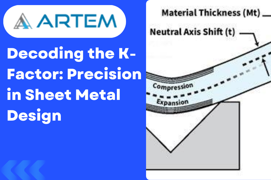
Welcome to the intricate world of sheet metal design, where precision is paramount, and every bend matters. In this blog, we’ll unravel the mystery behind a key player in sheet metal formulation: the K-Factor. Let’s explore what the K-Factor is, its significance in sheet metal bending, and how it dances in harmony with different materials. Understanding the K-Factor The K-Factor, short for “neutral axis factor” or “bend allowance factor,” is a critical parameter in sheet metal bending. It’s a dimensionless value that represents the ratio of the neutral axis location to the material thickness. In simpler terms, the K-Factor helps account for the material’s behavior during bending, ensuring accurate calculations for the flat pattern. The K-Factor Formula: A Glimpse into the Math The formula for calculating the K-Factor is: This distance is typically measured from the center of the material thickness to the neutral axis, where no stretching or compressing occurs during bending. Significance of K-Factor in Sheet Metal Bending Accurate Bend Allowance: The K-Factor plays a pivotal role in determining the bend allowance, which, in turn, influences the flat pattern’s accuracy. It helps adjust for the material’s stretching or compressing during the bending process. Material Behavior Consideration: Different materials exhibit varying behaviors during bending. The K-Factor provides a way to tailor the bending calculations to the specific characteristics of the material being used. Precision in Design: Achieving precision in sheet metal design is not just about angles and dimensions; it’s about understanding how the material responds to bending forces. The K-Factor ensures that your design aligns with the real-world behavior of the material. K-Factor and Material Relationship: A Symbiotic Dance The K-Factor is intricately linked to the material properties of the sheet metal being used. Different materials have distinct behaviors during bending, and the K-Factor allows designers to account for these variations. Here’s how the relationship unfolds: Material Ductility: Ductility, the ability of a material to undergo deformation without rupture or cracking, influences how the material stretches during bending. Materials with higher ductility might have different K-Factors compared to less ductile ones. Material Thickness: The thickness of the sheet metal also affects the bending process. Thicker materials may have different K-Factors compared to thinner ones, as the forces exerted during bending vary with thickness. Bend Radius: The radius of the bend significantly impacts the K-Factor. Different bend radii can result in variations in the stretching or compressing of the material, influencing the appropriate K-Factor to use. Conclusion: Mastering the Material Symphony In the realm of sheet metal design, the K-Factor is your guide to mastering the material symphony. It ensures that your designs are not just lines on paper but accurate representations of how the material will behave in the real world. As you delve into the world of sheet metal bending, remember that the K-Factor is your ally, helping you achieve precision, accuracy, and a harmonious dance between design and material reality. Happy bending!
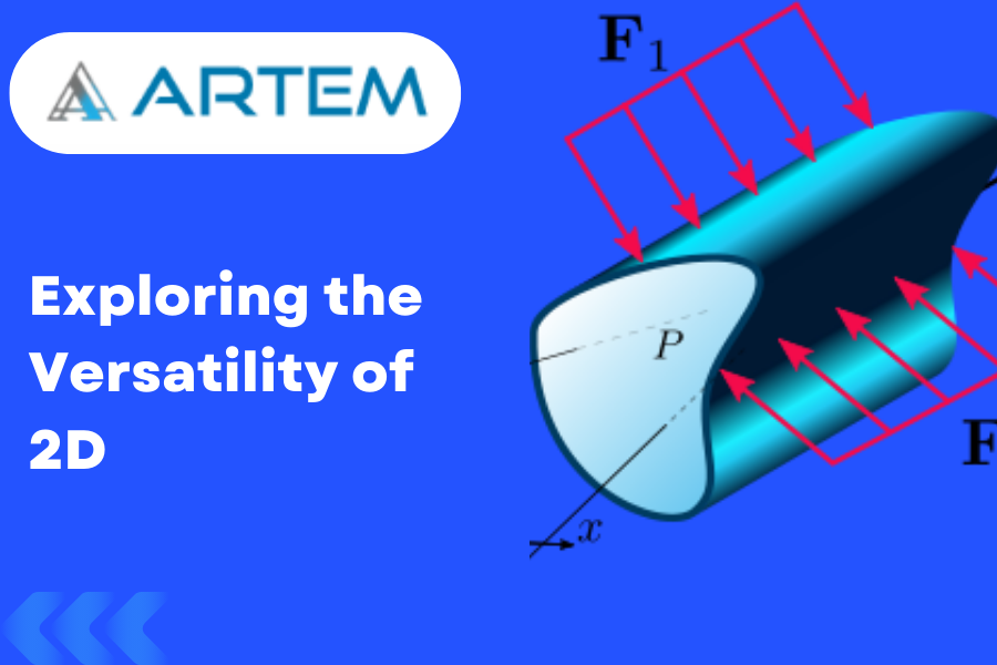
In Finite Element Analysis, the continuous domain is divided into a mesh of smaller subregions called elements, and each element is represented by a mathematical approximation referred to as a finite element. These elements are typically classified as one-dimensional (1D), two-dimensional (2D), or three-dimensional (3D), depending on the dimensionality of the problem being modeled. Specifically, 2D finite elements are used to discretize problems that exhibit behavior primarily in two dimensions, such as plane stress, plane strain, or axisymmetric problems. They are employed when the geometry and loading conditions can be adequately represented in a two-dimensional plane, and the third dimension can be neglected or approximated as a constant value. The shape and formulation of 2D finite elements can vary depending on the specific problem being addressed. Common types of 2D elements include triangular elements (e.g., linear or quadratic triangles) and quadrilateral elements (e.g., bilinear or biquadratic quadrilaterals). These elements are defined by a set of nodes and interpolation functions that approximate the behavior of the underlying continuous domain. The behavior of the structure or system can be analyzed, and quantities such as displacements, stresses, strains, and other relevant variables can be evaluated at specific points within each element. Overall, 2D elements in FEM provide a powerful numerical tool for analyzing and simulating the behavior of structures and systems in two-dimensional space, enabling engineers and researchers to gain insights into the mechanical response of various physical phenomena. Here is a detailed explanation of common types of 2D elements: 2D plane stress 2D plane stress refers to a simplified modeling approach used to analyze the behavior of a thin structure or component. It assumes that the stresses and strains within the structure are primarily confined to a single plane, neglecting the effects of stress and strain variations in the thickness direction. When considering the thickness element in a 2D plane stress analysis, it is assumed that the thickness of the structure is much smaller compared to its other dimensions. This assumption allows for the simplification of the analysis by reducing the problem from a 3D scenario to a 2D plane, where stress and strain components vary only within that plane. In this analysis, the structure is typically represented by a flat, two-dimensional model. The stresses and strains are assumed to vary only in the X and Y directions, while remaining constant in the Z (thickness) direction. This simplification allows for the application of two-dimensional equations of equilibrium and constitutive laws to determine the stresses, strains, and deformations within the structure. It is important to note that the 2D plane stress analysis is applicable only when the effects of stress variations in the thickness direction can be reasonably neglected. Overall, the 2D plane stress analysis with thickness element provides a simplified approach to analyze thin structures, allowing for efficient and practical analysis while capturing the essential behavior of the system within the plane of interest. 2D plane strain 2D plane strain element is a modeling approach used to analyze the behavior of a structure or component subjected to deformation in two dimensions while assuming no strain variations in the third dimension. It is typically employed when the structure or component is much larger in the third dimension compared to its thickness or other dimensions. The deformation and resulting strains within the structure are assumed to be primarily confined to a single plane, while negligible in the direction perpendicular to that plane. This assumption allows for simplification of the analysis by reducing the problem from a 3D scenario to a 2D plane, where strains vary only in the X and Y directions. The structure or component is typically represented by a two-dimensional model, where deformations and strains occur in the X and Y directions. The analysis involves applying two-dimensional equations of equilibrium and constitutive laws to determine the stresses, strains, and deformations within the structure. It is important to note that the 2D plane strain analysis is suitable when the strains in the direction perpendicular to the plane of interest are relatively small or negligible. This assumption is valid for structures or components that are significantly larger in one dimension compared to the other two dimensions, such as long beams, thick plates, or deep foundations. However, it is crucial to carefully consider the suitability of the 2D plane strain assumption for a given problem. If significant strain variations occur in the out-of-plane direction, a more comprehensive three-dimensional analysis may be necessary to accurately capture the behavior of the structure. In summary, a 2D plane strain element is a modeling technique used to analyze structures or components subjected to deformation in two dimensions while neglecting strain variations in the third dimension. It provides a practical and efficient approach for analyzing systems with predominant deformation occurring in a single plane. 2D Axi-Symmetric 2D axisymmetric element is a modeling approach used to analyze the behavior of a structure or component that possesses rotational symmetry around a central axis. It is particularly suitable for studying cylindrical or rotationally symmetric geometries, such as pipes, pressure vessels, or circular plates. In a 2D axisymmetric analysis, the deformation and resulting strains within the structure are assumed to be axisymmetric, meaning they vary only in the radial and axial directions. This assumption allows for a simplification of the analysis by reducing the problem from a 3D scenario to a 2D axisymmetric plane, eliminating the need to model the entire 3D volume. The structure or component is typically represented by a 2D axisymmetric model, where deformations, strains, and stresses are computed for points along the radial and axial directions. The analysis involves applying axisymmetric equilibrium equations and constitutive laws to determine the stresses, strains, and deformations within the structure. The boundary conditions applied to the model are also axisymmetric, and the loading conditions are assumed to be symmetrical about the central axis. This allows for the consideration of rotational symmetry and simplifies the analysis process. It is important to note that the 2D axisymmetric analysis is suitable when the geometry and
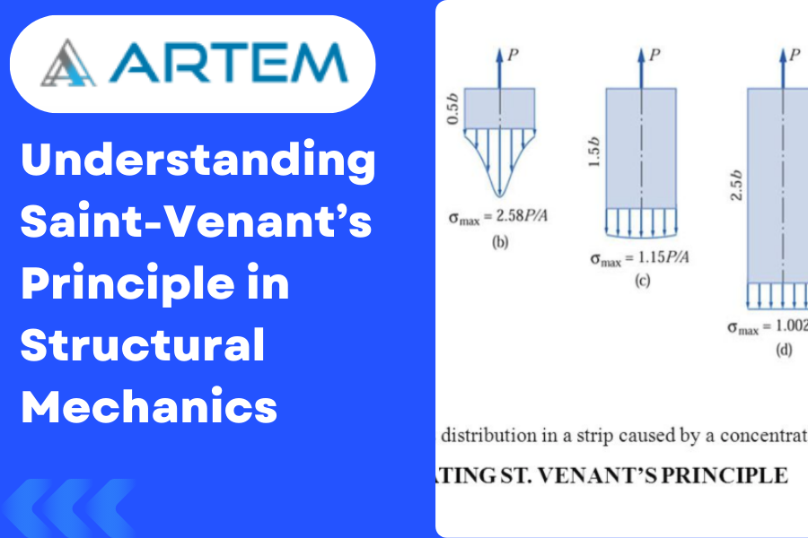
Saint-Venant’s Principle, named after the French engineer Adhémar Jean Claude Barré de Saint-Venant, is a concept in structural mechanics that provides guidance on how the distribution of stress becomes more uniform at a sufficient distance from a concentrated load or point of load application. The principle is particularly useful when analyzing the behavior of structures under localized loads. Saint-Venant’s Principle: Statement: “The stresses and displacements caused by the application of a concentrated load to a structural member become nearly constant at a sufficiently large distance away from the point of load application.” In simpler terms, as you move away from the point where a load is applied, the local effects of the load become less significant, and the behavior of the structure tends to become more uniform. Formula for Point Load Application: When applying a point load to a structural member, such as a beam, the distribution of stress and deformation can be determined using the equations derived from Saint-Venant’s Principle. For a simply supported beam subjected to a concentrated load at a point, the bending moment (M) and shear force (V) formulas at a distance x from the point of load application are given by: Bending Moment (M): $$ M(x)=P⋅(L-x)\;$$ where: P is the point load applied, L is the span length of the beam, x is the distance from the point of load application. Shear Force (V): $$V(x)=P$$The shear force remains constant along the length of the beam and is equal to the applied point load. Assumptions & Considerations: 1. Linear Elastic Material: Saint-Venant’s Principle is applicable to linear elastic materials, where the stress-strain relationship is linear. 2. Sufficient Distance: The principle becomes more accurate as you move a sufficient distance away from the point of load application. This distance is generally considered to be a few times the depth of the beam. 3. Uniformly Loaded Section: Saint-Venant’s Principle is more accurate for predicting the behavior of a section that is uniformly loaded. It is less accurate for predicting local effects near the point of load application. 4. Symmetrical Loading: For symmetrical loading conditions, Saint-Venant’s Principle tends to be more applicable. Application in Engineering: Saint-Venant’s Principle is widely used in engineering practice, particularly in structural analysis and design. It allows engineers to simplify complex loadings and assess the behavior of structures under more manageable conditions, especially when analyzing the effects of localized loads on beams and other structural elements. It’s important to note that while Saint-Venant’s Principle is a valuable tool, there are situations where its applicability may be limited, such as in regions close to the point of load application or in cases involving significant torsional effects. Engineers should be mindful of these limitations and use the principle judiciously in their analyses.