
Linear static analysis refers to a computational technique used in engineering and structural analysis to predict the response of a structure under applied loads or forces. It assumes linear relationships between applied loads and resulting displacements, as well as linear elastic material behavior within the structure. In linear static analysis, the governing equations of linear elasticity, such as the equilibrium equations and the stress-strain relationship described by Hooke’s law, are solved to determine the deformations, displacements, and internal forces within the structure. The analysis assumes small deformations, where the linear strain-displacement relationship holds, and it assumes that the material properties of the structure are homogeneous and isotropic. The analysis involves dividing the structure into smaller elements, typically finite elements, and solving the equilibrium equations for each element and the connections between them. The resulting system of linear equations is then solved using numerical techniques such as the finite element method (FEM) or other matrix-based methods to obtain the displacements and internal forces. Where K = Stiffness matrix U = Displacement Matrix F = Force Matrix Linear static analysis provides insights into the stresses, deformations, and displacement patterns within a structure, allowing engineers to evaluate its strength, stability, and safety. It is widely used in various fields, including civil engineering, mechanical engineering, aerospace engineering, and more, for designing and analyzing structures such as buildings, bridges, mechanical components, and assemblies. Importance of Linear Static Analysis Linear static analysis is a fundamental and widely used technique in engineering and structural analysis. It serves several important purposes and provides valuable insights into the behavior of structures. Here are some reasons highlighting the need and importance of linear static analysis: Predicting Structural Response: Linear static analysis helps predict the response of structures under various loading conditions. By analyzing the stresses, displacements, and deformations, engineers can assess the structural integrity and ensure that the design meets the desired criteria. It allows for evaluating the strength, stability, and safety of a structure. Design Validation and Optimization: Linear static analysis aids in the design validation process. Engineers can verify the performance of a structure by applying expected loads and studying the resulting behavior. It enables the identification of potential design flaws, weak points, and areas of excessive stress or deformation. This information can guide design optimization and modification to enhance the performance and efficiency of the structure. Load Distribution: Linear static analysis helps determine how loads are distributed within a structure. By studying the internal forces and stresses, engineers can understand how different components and members bear the load. This information is crucial for structural engineers to ensure that the load is properly distributed, and no individual component is subjected to excessive stress or overload. Material Selection: Linear static analysis facilitates material selection for a structure by evaluating stress levels and deformations. Engineers can assess the suitability of different materials based on their stiffness, strength, and other mechanical properties within the linear elastic range. ANSYS Workbench, a powerful engineering simulation software, can be used to analyze the mechanical behavior of structures. Learning ANSYS Workbench with Artem Academy can enhance engineers’ proficiency in utilizing this software for linear static analysis and other advanced engineering simulations. Artem Academy offers specialized courses that teach engineers how to effectively model and analyze structures, simulate various materials, and evaluate stress levels and deformations. By combining theoretical knowledge of material properties with practical application using ANSYS Workbench, engineers can confidently select materials that meet the specific requirements of a structure and can withstand anticipated loads and deformations within the linear elastic range. Support System Design: Linear static analysis aids in the design of support systems, such as beams, columns, and connections. By analyzing the internal forces and deformations, engineers can determine the required sizes, shapes, and configurations of support elements. This helps ensure the stability, rigidity, and proper load transfer within the structure. Cost and Time Savings: Linear static analysis allows engineers to assess different design alternatives quickly and cost-effectively. By simulating the behavior of a structure in a virtual environment, engineers can identify potential issues and make necessary modifications before physical prototypes or full-scale manufacturing. This iterative process saves time, reduces material waste, and minimizes the cost of physical testing and revisions. Overall, linear static analysis is a vital tool for engineers to understand and optimize the structural behavior of a wide range of systems. It provides valuable insights for design, validation, optimization, and ensuring the structural integrity and safety of various engineering projects.

Linear static analysis makes several assumptions to simplify the analysis of structures. These assumptions are necessary to apply the principles of linear elasticity and simplify the governing equations. Here are some common assumptions made in linear static analysis: Linear Elastic Material Behavior: Linear static analysis assumes that the material used in the structure exhibits linear elastic behavior. This means that the material obeys Hooke’s law, where the stress is directly proportional to the strain within the elastic limit. Nonlinear material behavior such as plasticity, creep, or large deformations is not considered in linear static analysis. Small Deformations: Linear static analysis assumes that the deformations in the structure are small. This assumption allows the use of the linear strain-displacement relationship, where the strain is directly proportional to the displacement. Large displacements that cause significant geometric changes and nonlinear effects are not considered in linear static analysis. Linear Relationship between Loads and Displacements: Linear static analysis assumes that the applied loads and resulting displacements have a linear relationship. This assumption implies that the structure’s response is directly proportional to the applied loads. It assumes that the superposition principle holds, meaning the response to multiple loads is the sum of the individual responses to each load. Static Equilibrium: Linear static analysis assumes that the structure is in a state of static equilibrium. This means that the applied loads and internal forces within the structure are balanced, resulting in zero net force and moment. Dynamic effects, such as inertial forces, are not considered in linear static analysis. Homogeneous and Isotropic Material: Linear static analysis assumes that the material properties of the structure are homogeneous (uniform throughout) and isotropic (properties do not vary with direction). This simplifies the analysis by assuming that the material behaves the same in all directions. Small Strain Theory: Linear static analysis employs the small strain theory, which assumes that the strains in the structure are small enough that the change in shape can be approximated by linear relationships. By making this assumption, the strain-displacement equations become simplified, facilitating the analysis process. At Artem Academy, we offer a comprehensive ANSYS course that covers the principles and applications of finite element analysis. Our course delves into various aspects of structural analysis, including linear static analysis. For more details, advanced analysis techniques, such as nonlinear analysis, may be required to accurately model the behavior of the structure .By enrolling in our ANSYS course online, students will gain a solid understanding of how to effectively utilize the ANSYS software to perform linear static analysis and other advanced simulations. Throughout the course, we explore the limitations of this theory and introduce more advanced analysis methods for scenarios where large strains or nonlinear behavior are involved. By providing a well-rounded education in structural analysis, our ANSYS course equips students with the necessary knowledge and skills to tackle complex engineering challenges. Whether you are a beginner seeking an introduction to ANSYS or an experienced professional looking to enhance your simulation capabilities, Artem Academy’s ANSYS course is designed to meet your needs. Join us today and take your engineering analysis skills to new heights.
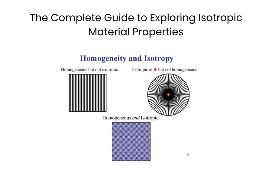
Isotropic material properties refer to the characteristics of a material that are independent of direction. In other words, their mechanical and physical characteristics, such as elasticity, thermal expansion, and conductivity, are the same regardless of the direction in which they are measured. Isotropic materials exhibit the same response to stress, strain, and other external factors, making their behavior predictable and uniform in all orientations. For example, consider a solid cube made of an isotropic material. When subjected to mechanical loading, the cube will deform uniformly in all directions, and the resulting stress and strain will be the same regardless of the orientation of the applied forces. That means, the response to applied forces or stimuli is the same regardless of the direction in which they are applied. For example, if a force is applied to an isotropic material along the x-axis, the resulting deformation or strain will be the same as if the force were applied along the y-axis or z-axis. Similarly, the thermal expansion and conductivity will be the same in all directions, and the material will exhibit the same electrical and magnetic properties in any direction. Homogeneous materials have uniform properties throughout their structure. This means that their composition and characteristics, such as density, composition, and mechanical properties, are consistent and identical in all regions. In other words, there are no variations or gradients in their material properties within the material itself. In summary, isotropic materials have consistent properties in all directions, while homogeneous materials have uniform properties throughout their structure without any variations or gradients. Here the details of material properties are mentioned below: Elastic Modulus: The elastic modulus, also known as Young’s modulus, is a measure of a material’s stiffness. In an isotropic material, the elastic modulus is the same in all directions, meaning it has the same resistance to deformation in any direction. Thermal Conductivity: Thermal conductivity is a property that describes a material’s ability to conduct heat. In an isotropic material, the thermal conductivity is uniform in all directions, meaning heat transfers at the same rate regardless of the direction of heat flow. Electrical Conductivity: Electrical conductivity refers to a material’s ability to conduct electric current. In an isotropic material, the electrical conductivity is the same in all directions, allowing for uniform electrical conduction throughout the material. Magnetic Permeability: Magnetic permeability is a measure of how easily a material can be magnetized in the presence of a magnetic field. In an isotropic material, the magnetic permeability is constant in all directions, indicating the same response to magnetic fields regardless of orientation. Density: Density represents the mass per unit volume of a material. In an isotropic material, the density remains the same regardless of the direction in which it is measured. These are just a few examples of isotropic material properties. It’s important to note that these properties are idealized assumptions and may not hold true for all materials in reality. Different materials can have varying degrees of isotropy or anisotropy, depending on their composition, crystal structure, and manufacturing processes. Isotropic material properties are represented by 2 independent variables i.e., Young’s modulus and Poisson’s ratio and is represented in equation as mentioned below form: Isotropic materials are often used as simplifying assumptions in engineering and scientific analyses because they are easier to work with mathematically and provide a good approximation for many practical applications. Common examples of isotropic materials include many metals (e.g., aluminum, steel), certain polymers, and some ceramic materials. Here are some common examples of isotropic materials: Glass: Most types of glass, such as window glass or soda-lime glass, are considered isotropic. They exhibit the same physical properties, such as optical transparency and mechanical strength, in all directions. Aluminum: Aluminum and its alloys, including commonly used ones like 6061 and 7075, are generally considered isotropic. They have consistent mechanical properties, such as stiffness and strength, in all directions. Polycarbonate: Polycarbonate is a transparent thermoplastic material widely used in applications such as safety glasses and bulletproof windows. It is isotropic and exhibits consistent properties throughout. Rubber: Certain rubber materials, such as natural rubber or synthetic elastomers like neoprene, can be considered isotropic. They possess similar properties in all directions, including elasticity and resilience. Polyethylene: Polyethylene, a widely used thermoplastic material, can exhibit isotropic behavior depending on its manufacturing process and grade. It is commonly used in packaging, pipes, and other applications. Acrylic: Acrylic, also known as PMMA (polymethyl methacrylate), is a transparent thermoplastic material that is often used as a substitute for glass. It is typically isotropic and has consistent properties in all directions. Isotropic materials are often used as simplifying assumptions in engineering and scientific analyses because they allow for easier calculations and predictions. Some examples of isotropic materials include many metals, certain polymers, and some ceramic materials. It’s important to note that while these materials are generally considered isotropic, specific manufacturing processes, additives, or material modifications can introduce some level of anisotropy in certain cases. Additionally, it’s always advisable to consult material specifications and conduct testing to confirm the isotropic behavior of a specific material.

Linear static analysis has numerous practical applications across various engineering disciplines. Here are some common practical examples mentioned: Structural Analysis: Linear static analysis is widely employed in structural engineering to evaluate the behavior of various structures, including buildings, bridges, towers, and other architectural elements. It helps determine the stresses, deformations, and displacement patterns under different loading conditions. Engineers can evaluate the strength and stability of structural components, optimize designs, and ensure compliance with safety regulations. Mechanical Component Design: This analysis is employed in the design of mechanical components such as machine parts, mechanisms, and industrial equipment. It helps evaluate the structural integrity and performance of components under applied loads. This analysis aids in optimizing component designs, identifying areas of excessive stress or deformation, and ensuring the functionality and reliability of the product. Automotive Industry: Linear static analysis plays a crucial role in automotive engineering. It helps assess the structural integrity and performance of vehicle components, such as chassis, frames, suspension systems, and body structures. This analysis aids in optimizing designs for weight reduction, improving vehicle safety, and ensuring durability under various operating conditions. Aerospace and Aircraft Design: In aerospace engineering, linear static analysis is used to analyze and optimize the structural behavior of aircraft components, such as wings, fuselages, and landing gear. It aids in assessing the structural integrity, load distribution, and stiffness of these components. Linear static analysis is also employed to study the interactions between different structural elements and evaluate their overall performance. Civil Engineering and Infrastructure: Linear static analysis is applied in civil engineering to analyze the behavior of structures like dams, tunnels, pipelines, and offshore structures. It helps evaluate the stability, load-carrying capacity, and safety of these structures under various loading conditions. Linear static analysis also aids in designing foundations, retaining walls, and other structural elements to ensure their stability and resistance to failure. Consumer Products and Industrial Machinery: Linear static analysis is an essential technique utilized in the design and optimization of consumer products like furniture, appliances, and electronic devices. It allows engineers to assess and ensure the structural integrity, load-bearing capacity, and overall safety of these products. Moreover, this type of analysis finds application in the analysis and design of industrial machinery and equipment, guaranteeing their structural soundness and reliability. Professionals in engineering fields, including those pursuing an ANSYS course in India, often rely on linear static analysis to understand the behavior of structures subjected to static loads. It enables them to optimize designs, evaluate performance, and ensure the safety and functionality of various systems and structures. Linear static analysis is just one type of analysis among many available, and it serves as a fundamental tool for engineers in their pursuit of design excellence and problem-solving.

Building Construction: 1D elements are used in structural engineering for analyzing and designing buildings. They help determine the behavior of beams, columns, and frames under different loading conditions, ensuring structural integrity and safety. Bridge Design: 1D elements are employed in the analysis and design of bridges, allowing engineers to assess the structural performance and behavior of bridge components, such as beams and trusses, under different loads and environmental conditions. Heat Exchangers: 1D elements are utilized in the design and analysis of heat exchangers, which are devices used for transferring heat between fluids. They help determine the temperature distribution and heat transfer rates within the exchanger, ensuring efficient heat exchange. Electrical Circuits: 1D elements, such as resistors, inductors, and capacitors, are crucial components in electrical circuit analysis. They enable engineers to understand the behavior and performance of circuits, such as power distribution systems, electronic devices, and communication networks. Environmental Studies: 1D elements are employed in environmental modeling to study the transport of pollutants, contaminants, or heat in different media, such as soil, water, or air. They assist in analyzing the dispersion and movement of substances, aiding environmental impact assessments and remediation strategies. These are just a few examples of the widespread applications of 1D finite elements in various engineering and scientific disciplines. The behavior of many systems can be effectively simplified as one-dimensional, allowing for efficient and accurate analysis using 1D finite elements. At Artem Academy, we offer comprehensive courses that cover not only 1D finite elements but also 2D and 3D models. In our blogs, we dive into the fascinating world of 2D and 3D finite element analysis, unveiling their applications in simulating and understanding complex systems. Whether you are dealing with structural mechanics, fluid dynamics, heat transfer, or electromagnetics, our blogs provide valuable insights into how to leverage 2D and 3D finite elements for accurate predictions and optimization. To develop your understanding and enhance your skills, we invite you to join our courses at Artem Academy. Our expert instructors will guide you through the theoretical foundations and practical aspects of finite element analysis, equipping you with the tools to tackle real-world engineering challenges confidently. From mastering meshing techniques to interpreting simulation results, our courses empower you to become a proficient analyst in 1D, 2D, and 3D simulations. Stay connected with our blogs, explore the diverse applications of finite element analysis, and embark on a transformative learning journey with Artem Academy.
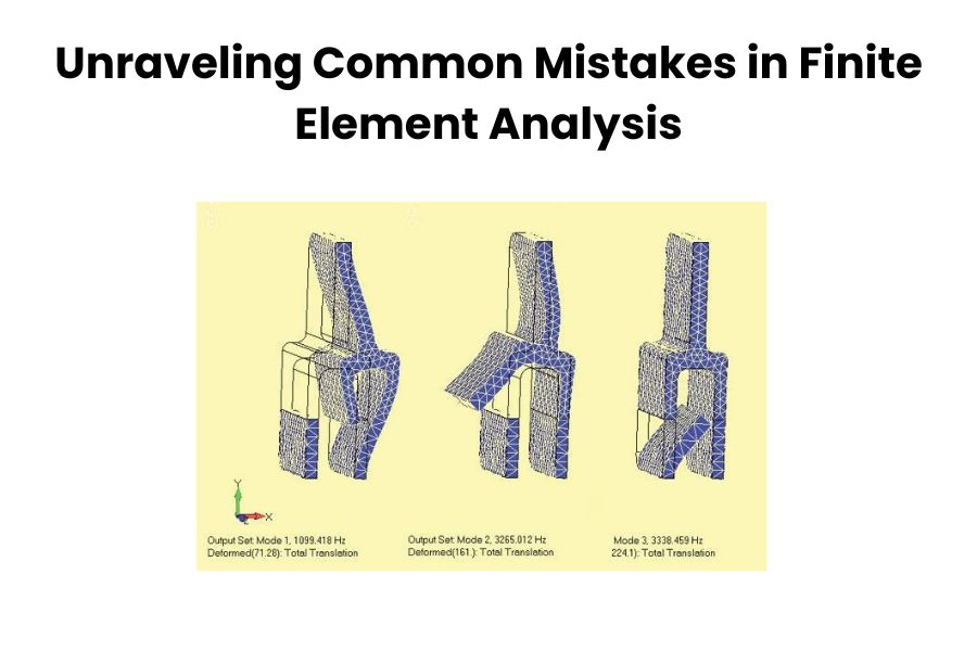
Finite Element Analysis (FEA) is one of the most powerful tools for analyzing and simulating simple to complex engineering problems in any industrial field. But cause of some common mistakes in Finite Element Analysis (FEA) can lead to inaccurate results and misleading interpretations. Some common mistakes that can occur during the FEA process are listed here: Incorrect Modeling: One of the common mistakes is not accurately representing the real-world geometry and boundary conditions in the FEA model. This can include missing or simplified features, incorrect material properties, or incorrect application of loads and constraints. It is crucial to carefully define the geometry, material properties, and boundary conditions to ensure accurate results. Insufficient Mesh Density: Using an insufficient mesh density can lead to inaccurate results, especially in areas of high stress gradients or regions where significant deformation occurs. It is important to ensure that the mesh is refined appropriately to capture the important features and variations in the solution accurately. Material properties: Another common mistake is using incorrect or inaccurate material properties in the FEA model. The material properties of the various types of material should be well-characterized and replication of the real-world behavior. In other words, it is essential to select appropriate material models based on experimental data or established material properties. Using inappropriate or outdated material properties can lead to misleading results. Neglecting boundary conditions: Accurate boundary conditions are crucial for obtaining meaningful results in FEA. Failing to apply the correct constraints or loads can lead to unrealistic or erroneous outcomes. It’s important to carefully define the boundary conditions based on the physical problem being analyzed. Neglecting mesh sensitivity analysis: The choice of mesh size and element type can significantly affect the accuracy of the FEA results. Neglecting to perform a mesh sensitivity analysis to determine the optimal mesh size can lead to either overly coarse or excessively refined meshes, impacting the accuracy and computational efficiency of the analysis. Neglecting Contact or Interaction Effects: In cases where contact or interaction between different components or surfaces is present, neglecting or improperly modeling these effects can lead to erroneous results. Properly defining contact conditions, including frictional or nonlinear behavior, is crucial to capture the correct behavior of the system. Convergence issues: FEA analyses often require iterative calculations to converge on a solution. Insufficient convergence criteria or inappropriate solution settings can result in non-converging analyses or inaccurate results. It’s important to carefully set up the solution parameters and monitor convergence to ensure reliable results. Overlooking Element Quality: Element distortion occurs when elements are excessively stretched, compressed, or distorted in some way. Poor element quality, such as highly distorted or poorly shaped elements, can result in inaccurate results. It is important to check for element quality metrics, such as aspect ratio, skewness, or Jacobian, and ensure that they meet acceptable criteria. Checking for element distortion and adjusting the mesh accordingly is crucial to obtaining reliable results. When working with ANSYS Workbench in India, it is essential to learn about element distortion, which refers to the excessive stretching, compression, or distortion of elements. Artem Academy is an excellent resource for learning ANSYS Workbench in India. It is important to evaluate element quality metrics such as aspect ratio, skewness, or Jacobian to ensure accurate results. By checking for element distortion and making necessary adjustments to the mesh, reliable and precise outcomes can be obtained. Ignoring model validation: It’s important to validate the FEA model against experimental data or known analytical solutions whenever possible. Neglecting model validation can result in a lack of confidence in the simulation results. Comparing the FEA results with experimental or analytical data helps identify and rectify any discrepancies or errors. Improper Interpretation of Results: Incorrect interpretation or overreliance on FEA results without considering limitations or assumptions can lead to incorrect design decisions. It is crucial to critically analyze and interpret the results while considering the underlying assumptions and limitations of the FEA model. Remember, FEA is a complex and iterative process, and attention to detail is crucial. To mitigate these mistakes, it is important to have a thorough understanding of the underlying theory and assumptions of FEA, pay attention to model setup and boundary conditions, verify results against experimental data or analytical solutions when available, and constantly validate and refine the FEA models based on real-world observations and feedback. Collaboration with experienced FEA analysts and seeking peer review can also help in identifying and rectifying potential mistakes. Also, by being mindful of these common mistakes and following best practices, engineers can improve the accuracy and reliability of their FEA simulations.

Element quality refers to the measure of how well an element represents the physical shape or behavior of the structure or system being analyzed. It provides an indication of the accuracy and reliability of the numerical results obtained from the finite element analysis (FEA). ANSYS uses various metrics to evaluate the element quality. Some commonly used measures include: Aspect ratio refers to the ratio of the longest edge or element size to the shortest edge or element size within a finite element mesh. It is used as a measure of the geometric quality of the mesh elements and can impact the accuracy and reliability of the analysis results. Aspect ratio is typically used as an indicator of mesh distortion or element shape irregularity. Ideally, elements in a mesh should have a reasonably uniform size and shape to accurately represent the geometry and avoid numerical issues. Mesh elements with poor aspect ratios can lead to numerical instability, inaccurate results, and difficulties in convergence during the analysis. The limits for acceptable aspect ratios depend on the type of elements being used and the specific analysis requirements. Here are some general guidelines: 1. Triangular Elements: For triangular elements, a commonly used quality measure is the ratio of the longest edge to the shortest edge. An aspect ratio close to 1 indicates nearly equilateral triangles, which are desirable for accuracy. In practice, aspect ratios up to 5 or 6 are often considered acceptable, but it is generally recommended to keep aspect ratios below 3 for well-conditioned elements. 2. Quadrilateral Elements: For quadrilateral elements, aspect ratio is defined as the ratio of the longest side to the shortest side. Similar to triangular elements, it is desirable to have nearly square or rectangular elements with aspect ratios close to 1. Acceptable limits for aspect ratios of quadrilateral elements typically range from 1 to 4 or 5, depending on the specific analysis and element type. It’s important to note that these aspect ratio limits are general guidelines and may vary depending on the specific analysis requirements, element type, and the software being used. In some cases, higher aspect ratios may be tolerated if they do not significantly affect the accuracy or stability of the analysis. In addition to aspect ratio, there are other mesh quality measures, such as element skewness, angle distortion, and element size variation, which should also be considered in assessing the overall mesh quality. Proper mesh refinement and optimization techniques can be employed to improve element quality and achieve a well-conditioned mesh for accurate and reliable finite element analysis. Warpage, also known as element distortion or element skewness, is a measure of the deviation from the ideal shape of a finite element. It quantifies the non-planarity or non-straightness of the element faces or edges. Warpage can affect the accuracy and convergence of finite element analysis results and is often considered in element quality checks. The warpage limit is a criterion that defines the maximum allowable warpage for an element to be considered acceptable. If an element exceeds the warpage limit, it is considered distorted and may lead to inaccurate or unreliable analysis results. The warpage limit is typically expressed as a dimensionless value or a percentage of the element size. The specific warpage limit depends on the element type, the analysis requirements, and the software being used. However, in general, a common guideline for triangular or quadrilateral elements is to keep the warpage below 0.2 or 20%. This means that the maximum deviation from the ideal shape should not exceed 20% of the element size. It’s important to note that the warpage limit is just one aspect of element quality checks, and other measures, such as aspect ratio, angle distortion, and element size variation, should also be considered. In practice, it is recommended to use a combination of quality measures to evaluate the overall quality of the mesh and ensure accurate and reliable analysis results. If elements exceed the warpage limit, mesh refinement techniques, such as element splitting or repositioning, can be applied to improve the element quality. Additionally, using higher-order elements or alternative element types may help reduce warpage and improve the accuracy of the analysis. Overall, maintaining low warpage within acceptable limits is important to ensure good element quality and reliable results in finite element analysis. Parallel deviation, also known as skewness or shape deviation, is a measure of how well the faces or edges of a finite element align with the ideal geometric shape. It quantifies the deviation from the ideal straightness or parallelism of the element edges or faces. Parallel deviation is an important aspect of element quality checks and can impact the accuracy and convergence of finite element analysis. The parallel deviation limit is a criterion that defines the maximum allowable deviation from parallelism for an element to be considered acceptable. If an element exceeds the parallel deviation limit, it is considered distorted, and it may introduce errors or instability in the analysis results. The parallel deviation limit is typically expressed as a dimensionless value or a percentage. The specific limit depends on the element type, the analysis requirements, and the software being used. However, a common guideline for triangular or quadrilateral elements is to keep the parallel deviation below 0.2 or 20%. This means that the maximum deviation from parallelism should not exceed 20% of the element size. It’s important to note that the parallel deviation limit is just one aspect of element quality checks, and other measures, such as aspect ratio, warpage, and element size variation, should also be considered. Evaluating multiple quality measures provides a comprehensive assessment of the mesh quality and ensures accurate and reliable analysis results. If elements exceed the parallel deviation limit, techniques such as element repositioning, mesh smoothing, or mesh refinement can be employed to improve the element quality. Additionally, using higher-order elements or alternative element types with better shape control can help reduce parallel deviation and improve the accuracy of the analysis. In summary, maintaining low parallel deviation within acceptable
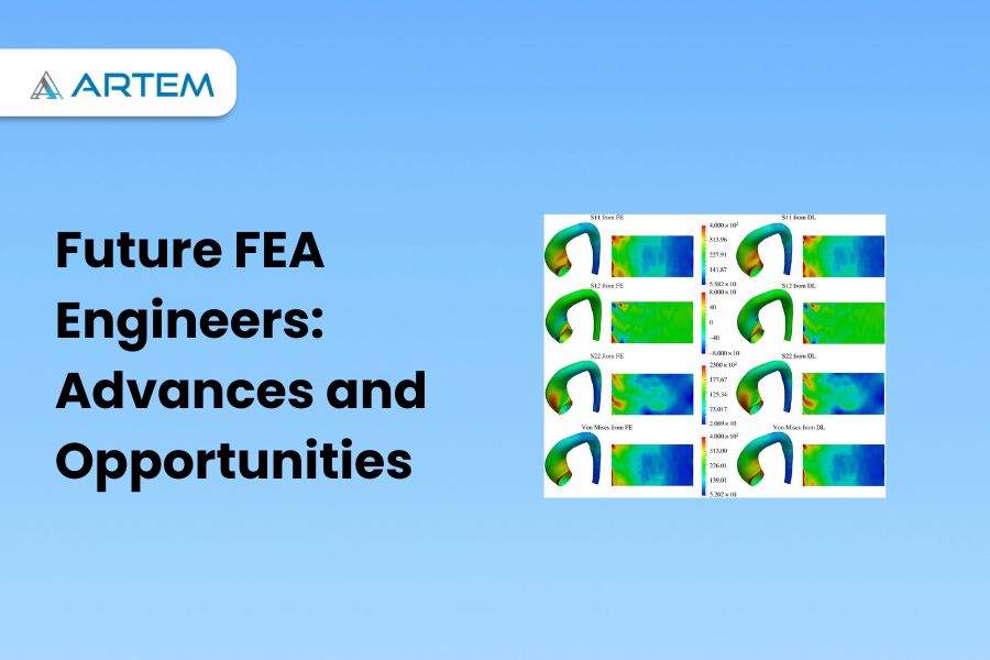
Finite Element Analysis (FEA) has been a powerful tool for engineering simulation for several decades. It has revolutionized the way engineers design and analyze structures, mechanical systems, and other products. However, as technology advances and computational power increases, the future of FEA looks even more promising. In this article, we will explore some of the emerging trends and technologies that are shaping the future of FEA. Artificial Intelligence (AI) and Machine Learning (ML) are revolutionizing the field of Finite Element Analysis (FEA). These technologies bring advanced capabilities and efficiency to FEA simulations. AI and ML techniques enable data-driven material characterization, automating the generation of FEA models, and adapting meshing based on stress distribution. They also facilitate predictive analysis, allowing engineers to forecast system behavior. Furthermore, AI can detect anomalies in simulation results, enhancing safety and reliability. ML-based optimization algorithms aid in design exploration, enabling engineers to efficiently explore design possibilities and find optimal solutions. The integration of AI and ML in FEA holds great potential for improving accuracy, accelerating processes, and driving innovation in engineering analysis. Cloud computing is transforming the field of Finite Element Analysis (FEA) by providing scalable, flexible, and accessible computational resources. With cloud computing, FEA engineers can leverage the power of remote servers and virtual infrastructure to perform complex simulations without the need for extensive local hardware or software installations. One of the key benefits of cloud computing in FEA is the ability to handle large-scale simulations. Cloud platforms offer high-performance computing capabilities, enabling engineers to solve computationally intensive FEA problems in a fraction of the time compared to traditional on-premises setups. This scalability allows for faster turnaround times and increased productivity in analyzing complex systems. Cloud-based FEA also promotes collaboration and remote work. Engineers can easily share simulation models, results, and analysis reports with team members, regardless of their geographical location. This facilitates efficient collaboration, enabling multiple experts to contribute to a project simultaneously and accelerating the overall development process. Another advantage of cloud computing is cost optimization. Instead of investing in expensive hardware and software licenses, FEA engineers can leverage cloud resources on a pay-as-you-go basis. Cloud service providers offer flexible pricing models, allowing users to scale resources up or down based on their specific needs. This approach reduces upfront costs and provides cost-efficiency for FEA projects, as users only pay for the resources they actually use. Furthermore, cloud computing enhances data management and security. Cloud platforms offer robust data storage, backup, and recovery options, ensuring the integrity and availability of FEA models and results. With proper access controls and encryption mechanisms, cloud providers maintain a high level of security, safeguarding sensitive engineering data. Overall, cloud computing revolutionizes FEA by providing on-demand computing power, enabling collaboration, optimizing costs, and enhancing data management and security. It empowers FEA engineers to tackle complex simulations efficiently and accelerates the overall engineering analysis workflow. High-Performance Computing (HPC) plays a crucial role in advancing the capabilities of Finite Element Analysis (FEA) by significantly accelerating the computational performance and enabling complex simulations. HPC refers to the use of powerful computing systems that harness parallel processing and massive data throughput to solve computationally intensive problems. FEA involves solving large systems of equations, which can be time-consuming for traditional computing resources. HPC provides a solution by distributing the workload across multiple processors or nodes, allowing for simultaneous computation and reducing the simulation time. This parallel processing capability empowers FEA engineers to tackle intricate models and perform parametric studies or design optimizations that were previously impractical or unfeasible. HPC also enables the handling of massive datasets involved in FEA simulations. With the ability to process large amounts of data in a shorter time, engineers can perform detailed analyses and capture more accurate results. This is particularly beneficial for simulations involving complex geometries, high mesh densities, or multi-physics phenomena. Additionally, HPC facilitates the exploration of design spaces and optimization in FEA. By leveraging the computational power of HPC clusters, engineers can efficiently evaluate multiple design iterations, perform sensitivity analyses, and conduct optimization studies. This empowers them to identify optimal solutions, enhance product performance, and streamline the design process. Furthermore, HPC allows for the integration of advanced simulation techniques, such as fluid-structure interaction, multi-scale analysis, or coupled physics simulations. These techniques involve complex algorithms and increased computational requirements, which are efficiently handled by HPC systems. This enables engineers to accurately simulate real-world scenarios and capture the interactions between different physical phenomena. In summary, HPC enhances FEA by significantly reducing simulation times, enabling complex simulations, handling large datasets, facilitating design exploration and optimization, and supporting advanced simulation techniques. By leveraging HPC resources, FEA engineers can push the boundaries of analysis capabilities, deliver more accurate results, and accelerate innovation in various fields, including aerospace, automotive, civil engineering, and more. Virtual Reality (VR) and Augmented Reality (AR) are emerging technologies that hold great potential for enhancing the field of Finite Element Analysis (FEA) by providing immersive visualization and interactive experiences. VR enables FEA engineers to step into a virtual environment where they can visualize and explore complex simulations in three dimensions. By wearing a VR headset, engineers can navigate through their FEA models, examine structural deformations, and observe the behavior of simulated systems from different perspectives. This immersive experience aids in understanding the intricate details of the analysis results, identifying potential issues, and gaining valuable insights into the behavior of structures. AR, on the other hand, overlays virtual information onto the real-world environment, allowing FEA engineers to visualize FEA results within their physical surroundings. With the help of AR-enabled devices, engineers can superimpose stress contours, displacement vectors, or other analysis data directly onto physical prototypes or real structures. This integration of virtual and real elements provides a contextual understanding of the FEA results, enabling engineers to compare simulations with physical reality and make more informed decisions. Both VR and AR technologies also facilitate collaborative design and analysis processes. FEA engineers can share their virtual environments or augmented views with team members or stakeholders, enabling them to collectively

Meshing can fail in ANSYS for several reasons, including geometry issues, element quality problems, improper mesh settings, and computational limitations. Here are some common reasons why meshing may fail in ANSYS: 1. Geometry issues refer to problems or anomalies present in the geometry that can hinder the meshing process or cause inaccuracies in the analysis. The issues need to be addressed before attempting to mesh the geometry are: Gaps and overlaps: Gaps occur when there are missing or disconnected surfaces in the geometry, while overlaps happen when surfaces intersect or occupy the same space. Gaps and overlaps prevent the creation of a watertight geometry, which is essential for proper meshing. These issues can result from errors in the CAD model or import process. To resolve them, you need to repair the geometry by closing gaps or removing overlaps using CAD software or Ansys’s geometry tools. Self-intersections: Self-intersections occur when surfaces or bodies intersect or penetrate each other within the geometry. Self-intersections can lead to invalid meshing as the meshing algorithm cannot handle overlapping or intersecting surfaces. It is necessary to identify and resolve self-intersections by modifying or repairing the geometry. Small features or sharp edges: Very small features or sharp edges in the geometry can pose challenges for meshing algorithms. Elements with extremely small sizes can cause meshing failures or lead to poor element quality. In such cases, it may be necessary to simplify or smooth out the geometry by removing unnecessary small details or rounding sharp edges. Thin or sliver surfaces: Thin or sliver surfaces are extremely thin regions in the geometry that can cause meshing difficulties. These surfaces may have a significantly different scale compared to the rest of the model, leading to meshing issues and poor element quality. It is advisable to address thin or sliver surfaces by thickening or removing them if they do not significantly impact the analysis. Complex or poorly defined geometries: Complex geometries with intricate details, sharp corners, or irregular shapes can be challenging to mesh accurately. Poorly defined geometries, lacking proper feature recognition or modeling, can also lead to difficulties in creating a high-quality mesh. In such cases, simplifying or partitioning the geometry and utilizing meshing techniques suitable for complex geometries can help overcome the issues. To address geometry issues: Review and repair the CAD model before importing it into Ansys. Use the geometry repair tools provided in Ansys to fix gaps, overlaps, or self-intersections. Simplify the geometry by removing unnecessary small features or rounding sharp edges. Identify and address thin or sliver surfaces by thickening or removing them if appropriate. Consider partitioning or simplifying complex geometries to facilitate meshing. Collaborate with CAD experts or consult ANSYS documentation and forums for specific guidance on resolving geometry-related issues. By addressing geometry issues, you can ensure a clean and well-defined geometry that facilitates successful meshing and accurate analysis in Ansys. 2. Element quality refers to the measure of the shape and quality of individual elements in a mesh generated in Ansys. High-quality elements are desirable as they ensure accurate and reliable results in finite element analysis. Poor element quality can lead to numerical inaccuracies, convergence difficulties, and unreliable simulation outcomes. Element quality metrics are used to assess the quality of elements within a mesh. Some common element quality metrics include aspect ratio, skewness, orthogonality, and Jacobian. These metrics provide quantitative measures of the element shape and distortion. Evaluate element quality using various tools and methods as mentioned below: Visualization: It provides visualization tools to examine the element quality visually. You can inspect the mesh and identify elements that exhibit poor shapes, such as distorted or highly stretched elements. Visual inspection allows you to identify problematic areas and focus on improving the mesh quality in those regions. Element quality criteria: Allows you to define specific element quality criteria or thresholds. You can set limits for metrics such as aspect ratio, skewness, and Jacobian to identify elements that fall outside the desired range. These criteria help in identifying elements that may adversely affect the accuracy of the analysis. Element quality checks: Ansys includes built-in checks and diagnostics to evaluate element quality. These checks identify problematic elements and provide diagnostic information to help pinpoint issues. For example, the software can flag elements with excessively high skewness or elements with very small aspect ratios. Mesh refinement: If poor element quality is identified in specific areas, you can refine the mesh in those regions. Mesh refinement involves reducing element sizes or employing adaptive meshing techniques to capture more detailed features or resolve distorted elements. Refining the mesh helps to improve element quality and ensures accurate representation of the geometry. By assessing and improving element quality, you can enhance the accuracy and reliability of the finite element analysis conducted. It is essential to maintain a balance between computational efficiency and mesh quality, ensuring that the mesh is fine enough to capture critical features while avoiding excessive computational costs. Inadequate mesh settings : lead to meshing failures or poor-quality meshes, which can adversely affect the accuracy and reliability of the analysis results. It is important to set appropriate meshing parameters to ensure a well-behaved and suitable mesh for the intended analysis. Here are some common inadequate mesh settings and their implications. Element size: The element size determines the level of mesh detail and accuracy. Inadequate element size settings can result in either a mesh that is too coarse, failing to capture important features and variations in the geometry, or a mesh that is too fine, leading to excessive computational costs. It is crucial to select an appropriate element size based on the geometry, analysis requirements, and the desired balance between accuracy and computational efficiency. Growth rate: The growth rate specifies how the element size increases or decreases as you move away from specified regions or boundaries. Inadequate growth rate settings can lead to abrupt transitions in element sizes or a lack of smooth gradation in the mesh. It is important to choose a suitable growth rate that ensures a smooth

A finite element method (FEM) is a numerical method used for solving engineering and mathematical problems involving the distribution of complex systems or structures into smaller, simpler, and interconnected subdomains. A set of mathematical equations approximates the behavior of each element. It has been widely applied in many fields, including structural analysis, heat transfer, fluid dynamics, and electromagnetics. The history of the Finite Element Method dates back to the early 1940s, with the work of Richard Courant, a German mathematician. Courant, along with his collaborators, developed a numerical technique called the Ritz-Galerkin method for approximating solutions to differential equations. This method laid the foundation for what would later become the Finite Element Method. In the late 1950s, engineers and mathematicians began developing the concept of dividing structures into small subdomains to simplify analysis. Notable pioneers in the development of FEM during this time include J.H. Argyris, Ray W. Clough, and Olek Zienkiewicz. They published seminal papers outlining the mathematical foundations and practical applications of the method. The first recorded use of the term “finite element” in the context of structural analysis dates back to the 1960s. It was coined by two engineers, Ray W. Clough and G. Temple, in their 1965 paper titled “The Finite Element Method in Plane Stress Analysis.” In this paper, Clough and Temple described their approach to solving plane stress analysis problems using a numerical method they referred to as the “finite element method.” They introduced the concept of dividing the domain into small subdomains (finite elements) and deriving the governing equations for each element. The authors highlighted the benefits of this method, including its ability to handle irregular geometries and complex boundary conditions. Since then, the term “finite element” has become the widely accepted terminology for this numerical technique, and it has been used consistently in subsequent research papers, books, and software development related to the method. The first book on the finite element method was “The Mathematical Foundations of the Finite Element Method” by Jacques Louis Lions and Olgierd C. Zienkiewicz. It was published in 1972. This book provided a comprehensive mathematical treatment of the finite element method, outlining the underlying principles and mathematical formulations involved in solving problems using the method. It became a seminal reference for researchers and practitioners in the field and played a significant role in the popularization and advancement of the finite element method. In 1960, Zienkiewicz, a British engineer, published a landmark paper titled “The Finite Element Method in Structural and Continuum Mechanics,” which introduced the term “finite element method” and presented the formulation of the method for structural analysis. Zienkiewicz’s work helped popularize the method and laid the groundwork for its subsequent development and application in various fields. The first finite element software was developed by a team led by Richard H. Gallagher at the Structural Analysis Group at the University of California, Berkeley. The software, known as STRESS, was created in the early 1960s and was primarily used for structural analysis. STRESS was one of the earliest implementations of the finite element method and was initially developed for linear elasticity problems. It allowed engineers to input the geometry, material properties, and boundary conditions of a structure and then perform stress analysis calculations using the finite element method. The software utilized the matrix displacement method, which is a precursor to the more widely used displacement-based formulation. While STRESS was significant in pioneering the application of the finite element method, it was a relatively simple program compared to modern finite element software packages. Over the years, the development of commercial software such as NASTRAN, ABAQUS, ANSYS, and many others has greatly expanded the capabilities and applications of the finite element method. Expansion and Diversification: Throughout the 1970s and 1980s, the finite element method expanded rapidly into various fields of engineering and science. Researchers extended its applications to areas such as heat transfer, fluid dynamics, and electromagnetics. The method’s flexibility and ability to handle complex geometries and boundary conditions contributed to its popularity. Advancements and Refinements: Over the years, researchers have continually refined and enhanced the finite element method. The development of powerful computers in the latter half of the 20th century greatly accelerated the progress of the Finite Element Method. The availability of computational resources enabled engineers and scientists to solve more complex problems and perform more accurate simulations. Commercial software packages dedicated to finite element analysis (FEA) emerged, making the method more accessible and practical for engineering applications. Since its inception, the Finite Element Method has continued to evolve, with improvements in element formulations, numerical algorithms, and computer hardware. It has become a standard tool in engineering and scientific communities, offering efficient and accurate solutions for a wide range of problems involving structural, thermal, fluid, and electromagnetic analyses. Today, the Finite Element Method remains a prominent and indispensable numerical technique, widely used in industries such as aerospace, automotive, civil engineering, and biomechanics, among others. Its versatility and robustness have made it a cornerstone of modern computational engineering and analysis.